MAT2500 16S [Jantzen] homework and daily class log

Your homework will appear here each day as it is assigned, with occasional links to some MAPLE worksheets when helpful to illustrate some points where technology can be useful. [There are 56 class days in the semester, numbered consecutively below and labeled by the (first initial of the) day of the week.]

It is your responsibility to check homework here. (Put a favorite in your browser to the class homepage.) You are responsible for any hyperlinked material here as well as requesting any handouts or returned tests or quizzes from classes you missed. Homework is understood to be done by the next class meeting (unless that class is a test, in which case the homework is due the following class meeting). WebAssign deadlines are at 11:59pm of the day they are due, allowing you to complete problems you have trouble with after class discussion.

*asterisk marked problems are to be done with MAPLE as explained in the separate but still tentative MAPLE homework log, which will be edited as we go.

Textbook technology: WebAssign homework management/grading is required, giving you access to an incredible wealth of multimedia tools together with the online e-book textbook you can access from any internet connection. Problems which are not available in WebAssign will be square bracketed and must be done outside of WebAssign. Problem numbers in red indicate a tutor help link in the textbook.

M (January 11, 2016):
GETTING STARTED STUFF. By Wednesday, January 13, reply to my welcome e-mail [robert.jantzen@villanova.edu] sent to your OFFICIAL Villanova e-mail account (which identifies you with your full name), telling me about your last math courses, your comfort level with graphing calculators and computers and math itself, [for sophomores only] how much experience you have with Maple (and Mathcad if appropriate) so far, why you chose your major, etc, anything you want to let me know about yourself. Tell me what your previous math course(s) was(were) named (Mat1500 = Calc 1, Mat1505 = Calc 2, Mat2705 = DEwLA).
HINT: Just reply to the welcome email I sent you before classes started.
[In ALL email to me, include the string "mat2500" somewhere in the subject heading if you want me to read it. I filter my email.]

On your laptop/tablet if you brought it:
1) Open Internet Explorer or your favorite browser. (You can open Maple files linked to web pages automatically if Maple is installed on your computer.)
2) Log in to MyNova on the Villanova home page in a browser (click on the upper right "login" icon and use your standard VU email username and password) and check out our class photo roster in the Student tab, and visit the link to my course homepage from it by clicking on my home page URL under my photo and then on our class homepage, directly (better yet, right click on the link and open it in another tab to get rid the MyNova header at the top of the window!):
[ http://www.homepage.villanova.edu/robert.jantzen/courses/mat2500/ ],
3) Open Maple if you already have it by clicking on this maple file link: bloodflow.mw
And then bob will then set the stage for 12.1, and open a handwrittten PDF solution and Maple solution of a multistep problem in the handouts folder linked to our course home page to demonstrate multistep problems [12.1.44,45,46].
4) bob will quickly show you the computer environment supporting our class.
[maybe he will try to impress you with this gee whizz! Maple video; naahh...we'll leave this only to the curious among us.]

During class in the first part of the semester, a signup sheet will be passed around for your signature. Make sure you sign at the end if it bypasses you. Today please put your nickname or your first name to be used in class, and include your cell phone number and your 3 letter dorm abbreviation listed on the short list side of the signup sheet.

log on to My Nova, choose the Student tab, click on the double person icon to the right of our class line to get to our photo class roster [look at the photo class roster to identify your neighbors in class!]
and click on my home page URL under my photo. Click on our class URL there. Check out the on-line links describing aspects of the course (no need yet to look at the MAPLE stuff).
[You can drop by my office St Aug 370 (third floor, Mendel side, by side stairwell) to talk with me about the course if you wish and to see where you can find me in the future when you need to.]

Homework (light first day assignment):
Make sure you read my welcoming email sent on the weekend (and reply to it within a few days), and register with WebAssign (immediately, if not already done).
Explore the on-line resources. Read the pages linked to our class home page. [Read computer classroom /laptop etiquette.]
Fill out the paper schedule form bob handed out in class [see handouts]; use the 3 letter dorm abbreviations to return in class the next class day.

Look over the class paper handout on diff/int/algebra.

WebAssign Problems: WebAssign101 is a very quick intro to WebAssign due Tuesday midnight;
read 12.1 reviewing 3d Cartesian coordinate systems, distance formula and equations of spheres [example];
12.1: 23, 45 (short list so you can check out our class website and read about the course rules, advice, bob FAQ, etc, respond with your email; those who do not yet have the book should be using the e-book through WebAssign. It is important that you read the section in the book from which homework problems have been selected before attempting them. Here is an example of a PDF problem solution: Stewart 12.1.46 [Okay, I cheated and looked at the solution manual to see how to get started. Then I made a nice Maple worksheet of the problem, just to have an example of a Maple worksheet to show you. Don't worry, we will take it slow with Maple.]

Download Maple 2015 if you haven't already done so and install it on your laptop when you get a chance (it takes about 15 minutes or less total), I will help you in my office if you wish.). If you have any trouble, email me with an explanation of the errors.
You are expected to be able to use Maple on your laptop when needed. We will develop the experience as we go. No problem if you never used it before.
W: return your schedule forms at the beginning of class;
check cell phone number, dorm info on daily signup sheet from first day entry;
12.1: 11, 15, 17, [19a hint: show the distance from P₁ to M is the same as from P₂ to M and equal to half the total distance; this is the hard way with points and not vectors],
12.2: 1, [2], 3, 5, 7, 13, 15, 19, 21, 25, 29.
Th: Office hours and course info document handout;
12.2: vector diagram problems [numbers for example 7];
34 (draw a picture, express the components of each vector, add them exactly (symbolically), evaluate to decimal numbers, think significant digits),
37 [same as example 7, different numbers],
45 [grid].
F: Quiz 0 on 12.1 [not graded, but due Wednesday in class for feedback on your presentation].
12.3 dot product: [example 3];
1, 2, 5, 9, 11, 15, 21, 23, 33;
optional fun problems if you like math: [55] (geometry [pdf,.mw]),
[57] (chemical geometry [ soln.mw, plot: methane.mw]).

WEEK 2[-1]:
M: no class, MLK Day.
W: turn in Quiz 0;
handout on resolving a vector and read this Maple worksheet: [using Maple (for dot and cross products and projection)];
12.3 projection: 39, 41, [45], 46, 49.
Th: Quiz 0 answer key on line---please examine carefully for presentation;
12.4 cross product: handout on geometric definition;
[why component and geometric definitions agree: crossprodetails.pdf];
1, 7, 11, 13, 16, 19, 27 (find 2 edge vectors from a mutual corner first, use 3 vectors and cross product),
31 (Maple example: trianglearea.mw),
33, 35, 37 (zero triple scalar product => zero volume => coplanar),
39 (first redo diagram with same initial points for F and r).
[54, why are a) and b) obvious? visualization]

Note:
> <2,1,1> · (<1,-1,2> x <0,-2,3>)
[boldface "times" sign and boldface centered "dot" from Common Symbols palette parentheses required]
> <2,1,1> · <2,1,1> then take sqrt (Expressions palette) to get length [example worksheet: babyvectorops.mw]

ignore this: [triplecrossproduct identity?]
F: Quiz 1 thru 12.3 ; it is helpful to bring a straight edge to draw lines;
[look at quiz archive 2500 14S to get an idea what I expect, given any two vectors in the plane, one can project one along and perpendicular to the other];
we can even make an animation of this with a little extra care showing both the acute and obtuse included angle case for the projection:
handouts/triangleprojectionvideo.gif [.mw];

detour: parametrized curves (online handout only; oops needs correction next week 3/2 power not 2/3!):
[textbook example curves: s10-1.mw (wow!)][parametrized curve tutorial];
open these worksheets and execute them by hitting the !!! icon on the toolbar (then read them!);
it is not very useful to try to draw parametrized curves based on what the graphs of x and y look like: technology is meant for visualizing math!;
BUT REMEMBER, WE JUST NEED TO WORK WITH SIMPLE CURVES.
10.1: 4, 9, 13, 17 [hyperbolic functions, Stewart 8e section 3.11: cosh² x- sinh² x = 1, recognition is enough],
21, just for fun: [28: eqns; it does not hurt to use technology if you cannot guess them all];
33, [37].

> plot([cos(t), sin(t)], t =0..2)           square bracket after last function, plots functions versus t on same axis
> plot([cos(t), sin(t), t =0..2])           square bracket after parameter range, plots parametrized curve in plane
or
> cos(t), sin(t)   right click on output, choose Plots, PlotBuilder, 2d parametrized curve (3d for curves in space).

Snowmaggedon!

WEEK 3[-1]:
come visit me 5 minutes in my office during weeks 3, 4, 5,
the sooner the better if you are having any troubles
[test 1 on chapters 12, 13 in week 5]
M: Snow Day, but you still have to work:
read online the handout on lines and planes [.mw];
never use the symmetric equations of a line: they are useless for all practical purposes!;
12.5: 1 (draw a quick sketch to understand each statement),
3, 5, 7 (parametric only),
13, 16, 19; 24, 31, 41, 45, 51 , 57[.mw].
W: class roster handout (paper only)---let's try to find one or two (preferable) partners for Maple assignments;
handout on geometry of points, lines and planes (distances between);
in these problems do not just plug into a formula: this is practice in vector projection geometry, we really don't care about the distance!:
12.5: 69 (DO NOT PLUG into FORMULA, find point on line, project their difference vector perpedicular to the line as in handout),
71 (find point on plane, project their difference along the normal) ,
73 (find pt on each plane, project their difference vector along the normal);
76 (draw a figure, find a point on the plane and move from it along the normal in both directions to get a point in the two desired parallel planes),
78 [.mw finding the closest points!] (find pt on each line (set parameters to zero!), project the 2 point difference vector along the normal to the parallel planes that contain them; ans: D = 2);
[optional challenge problem: 81].
Th: 12:R (Review problems are not in WebAssign): 24, 25, 26, 38;
read section 12.6 only for fun, since we will be using quadric surfaces during the course so why not skim through this material quickly?;
For fun (to stretch your thinking about multivariable equations), consider 13.1:21-26, trying to correlate aspects of the expressions for the coordinates with the spacecurve they determine, by matching one by one parametrized equations and graph.
F: Quiz 2 on eqns of lines and planes through Wed HW, dot/cross product applications;
Maple assignments start (read these instructions): note asterisks;
13.1: [cubic, cutcylinder] [1], 3,[5], 7, 13, 21, 25 [21-26, do quickly by thinking, note technology is not necessary here to distinguish the different formulas: .mw],
27, 33, [39*: refer back to similar problem 27: note that z² = (x²+y²)! plot the spacecurve and the surface together as in the template, adjust the ranges for the surface so it is just contains the curve and it not a lot bigger;clue: look at boxed axes ranges for the curve to chose your winow for the surface];
43 [eliminate z first by setting: z² (for cone) = z² (for plane) and solve for y in terms of x, and then express z in terms of x and finally let x be t; Maple can solve the pair of equations for {y,z} in terms of x],
[12.5.57*: using the answer in the back of the book and this template, plot the two planes and the line of intersection and confirm that visually it looks right. Adjust your plot to be pleasing, i.e., so the line segment is roughly a bit bigger than the intersecting planes (choosing the range of values for t)].

WEEK 4[-1]:
M: 13.2 : [in class: 1: pdf, 2], 5 [recall: exp(2t) = (exp(t))², what kind of curve is this?], 7, 10, 15, 19, 21, 31, 29a (by hand),
29b* [graph your results using this tangent line template; make a comment about how it looks].

on-line handout: key idea of vector-valued functions and the tangent vector (see Maple video: handouts/secantlinevideo.mw);
Maple stuff:
> with(Student[VectorCalculus]):               or Menu: Tools, Load Package, Student Vector Calculus
> <1,2,-3> × <1,1,1>
                 5 e_x - 4 e_y - e_z
[this is just new notation for the unit vectors i, j, k; > BasisFormat(false): returns to column notation]
> F := t → <t, t² , t³> : F(t)
> F '(t)
> ∫ F(t) dt
> with(plots):
> spacecurve(F(t), t=0..1, axes=boxed)
or just
> t, t² , t³
then Right Click, Plots, Plot Builder, 3d parametric curve (also for 2d parametric curves with 2 expressions);
and recall for 2D plots:

> plot([cos(t), sin(t)], t =0..2)           square bracket after last function, plots functions versus t on same axis
> plot([cos(t), sin(t), t =0..2])           square bracket after parameter range, plots parametrized curve in plane
W: 13.2: 22 [check your answers against Maple worksheet],
33 [angle between tangent vectors],
39 [use technology to do the integrals],
[43], 48, 49,[54, use combined dot/cross product differentiation rules 4,5 from this section:
(a · (b x c)) ' = a' · (b x c)) + a · (b' x c)) + a · (b x c')) ].
[product rule holds for all the products involving vector factors as long as you keep the order of factors the same in each resulting term if cross products are involved; usual sum rules always apply]
Th: 13.3: arclength toy problems require squared length of tangent vector to be a perfect square to be integrable usually! [or a factorization that makes a u-sub work!] [WebAssign for Friday but due date Monday night in case we cannot discuss HW Friday]
handout on arclength and arclength parametrization;
3 [note the input of the sqrt in the integrand is a perfect square in this problem];
5, [note the factorization to make an obvious u-sub];
10 [use numerical integration either with your graphing calculator or if you use Maple, right-click on output of integral, choose "Approximate";
for the curious: oops! what a mess!];
11 [hint: to parametrize the curve, first express y and then z in terms of x, then let x = t; another perfect square],
12 [hint: let x = cos(t), y = 2 sin(t) for the ellipse, then solve the plane eqn for z to get the parametrization, for one revolution of this ellipse]
F: Quiz 3 on 13.1-2; Test 1 next Thursday;
13.3 (curvature): handouts on geometry of spacecurves (page 1 for 13.3) and space curve curvature and acceleration (pages 2-3 for 13.4 later, 4 for both, print together);
[example Maple worksheets on these handouts: rescaled twisted cubic (page 1), helix (page4)]
13.3: 17, 25,
27 [do not use formula 11: instead use the parametrized curve form r = <t,t⁴,0> of the curve y = x⁴, then let t = x to compare with back of book or to enter in WebAssign];
47 [twisted cubic: perfect square!], 49; 51 [standard eqn: x²/9+y²/4 = 1, so r = <3 cos(t),2 sin(t),0>].

> with(Student[VectorCalculus]):
SpaceCurveTutor(<t,t²,0>,t=-1..1) from the Tools Menu, Tutors, Vector Calculus, Space Curves [choose animate osculating circles]
2d parabola osculating circle zoom.

show and tell 2d curves: osculate-parabola.mw, osculate-ellipse.mw

WEEK 5[-1]:
M: 13.4 (no Kepler's laws): 1, [2 avg velocity = vector displacement / time interval],
5, 11 [recall v = exp(t) + exp(-t) since v² is a perfect square],
17a, 17b*[graph your spacecurve using the template; pick the time interval t = -n π..n π, where n is a small integer, and by trial and error, reproduce the figure in the back of the book with 6 peaks, rotating the curve around and comparing with the back of the book sketch (note the horizontal axis tickmarks); if you wish, then animate the curve with the template provided],
[37 note that v² = 3²(1 + t²)² is a perfect square],
39,
[41? also perfect square, see 11] , 45 [visualize it!]

optional on-line only: osculating circle, how to describe mathematically using vector algebra.
W: online only: projections revisited just for those who like vector geometry;
on-line reminder of dot and cross products and length, area, volume;

13.4: 19 (minimize a function when its derivative is zero (critical point)! confirm minimum by plotting function);
13.R. (p.874-875):
[14a: use parametrized curve r = [t, t⁴- t²,0], evaluate T '(0) before simplifying derivative (i.e., set t = 0 before simplifying the expressions after differentiating) to find N(0) easily, find osc circle: x² + (y+1/2)² = 1/4],
14b*: edit the template with your hand results including comments and also do the zoom plot to see the close match of the circle to the curve];

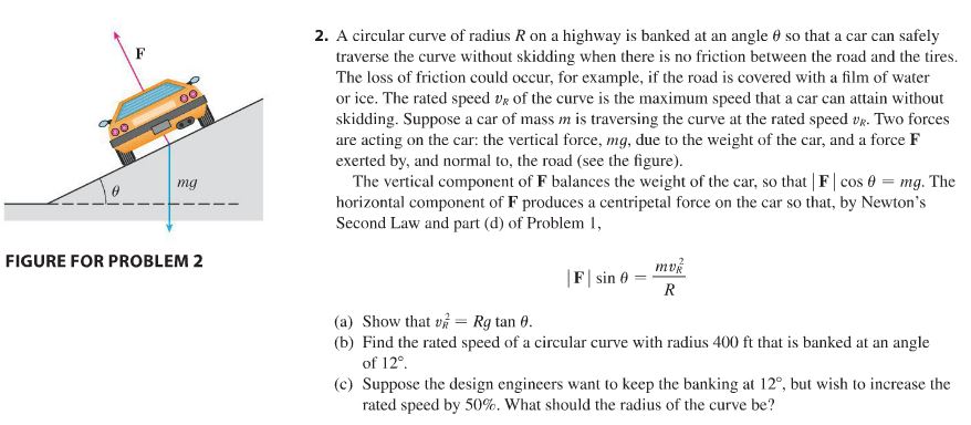
This is the most interesting HW problem (in class work): [Problems Plus 2. Note b) has answer 52 ft/sec = 36 mph; read about it].

Maple 13 is due any time next week; did you do your 5 minute office visit?

5:30pm MLRC voluntary problem session for Test 1.
Th: TEST 1.
F: no quizzes during test weeks. Maple workshop today to get a head start on Maple13.mw.
Download Maple13.mw and get started helping each other. Read the instructions on the Maple HW page.

Valentine's Day: good but better!
[Maple: heart.mw]

WEEK 6[-1]:
M: 14.1: 1, 3, 11, 15, 25, 31, [33], 35, 41, 49;
|maple14.mw problems begin:
55*, using this template just do a single appropriate plot3d and contourplot after loading plots and defining the maple function f (x,y)],
81a (read only b,c; if you are interested to see how the data is fit see example 3 among the interesting examples from 14.1 shown in Maple);
after finishing the preceding, for fun only look at 61-66 (maple plots reveal relationships, try to see correlations between formulas and 3d plots, then the contourplots).
W: 14.2: [1], 2, [4, 5], 9, 13, [15], 17,
23* [toolbar plot option: contour, or "style=surfacecontour" or right-click style "surface with contour", explain in comment],
25, 31, 37* [does a 3d plot of the expression support your conclusion? that is, your conclusion drawn before looking at the back of the book obviously, plot and explain], 39.
Th: finally partial derivatives! 14.3: [1], 3, 5, 11, 15, 17, 21, 31, 33, 41, 51 [in class if time: 22, 24, 28, 30].
F: no quiz yet;
14.3: second and higher derivatives (and implicit differentiation!) 47, 49; 53, 56, 59, 63, 65 [use this example for higher derivatives];
73 [just average the adjacent secant line slopes on either side of the point where the partial derivative is to be evaluated, as in the opening example: pdf, this is not a testing problem! tedious so I show you how to work through it],
[81], 83, [84, 88 ideal gas law], 90.

Test 1 back. Read Test 1 Answer key. Read test rules and academic integrity link. No future tests will be graded without signed pledge.
Check Blackboard grades against your paper grades in case I made an entry error.

WEEK 7[-1]:
M: 14.4: (linear approximation and tangent planes: differentiability illustrated): 1, 3, [7,] 11, [15], 17, 21, 22 [.mw].
7*[calculate by hand, then do two plots: first > plot3d( [f(x,y),L(x,y)],x = a..b, y = c..d); choose appropriate ranges centered about the point of tangency to show a good part of the surface behavior together with the tangent plane, then zoom in by choosing a smaller window about the point of tangency as instructed by the textbook, check that they agree, make a comment that it looks right confirming differentiability].
online handout on linear approximation and differentials (page 1 today, page 2 next class).
W: Quiz 4 on 14.3;
14.4 (differential approximation, error estimation): 25, 27, 31, 33, 35, 38, 39 [remember partials of this function from 14.3.83]; extra:
In the USA (inch units), the 4x6 photo prints have dimensions 4 in by 6 in. In Europe (cm units) the 10x15 prints have dimensions 10cm by 15 cm. Unit conversion: 1 inch = 2.54 cm. Use the differential approximation to estimate the absolute change and percentage change in the (computed) area of the USA format (new) compared to the European format (old): A = x y . Then compare your linear estimates for both to the corresponding exact changes. [HINT: apply the differential approximation using the x and y values of the European format, with the differentials dx and dy given by the differences USA format dimensions minus the European dimensions.] [Solution: 4x6prints.mw]
Th: 14.5: chain rule: 1, 11, 15, 17 (I never use tree diagrams), 21, 31 31 (no need to remember these equations, just implicit differentiate and solve in practice), 35, 39.
F: work on Maple14.mw;
14.5: 41 [units?], 43 [in degrees per second?], [these are important: 45: pdf, 49].
optional: [53] [just read this to see how it works if you are interested: maple, pdf; note this "coordinate transformation" of this second order derivative expression is extremely important for gravitational, electromagnetic, quantum mechanical and heat transfer problems, among many others].
Try one of these without looking at the soln or try 50.

Problem 49 describes waves: the wave equation for 1 d traveling waves.
Fun: Stephen Colbert Briane Greene 8 minute summary of the exciting gravitational wave discovery on the 100th anniversary of the Einstein equations for gravitation: our mathematical universe illustrated.

SPRING BREAK! Enjoy. Be safe in your travels.

WEEK 8[-1]: [note you can enter the page A127 in the e-book to get immediately to the current odd problem answers for 14.6]
M: 14.6 (directional derivatives; stop at tangent planes): 1, 3, 5, 7, 9, 11, 15,
19 [first find a unit vector in the given direction! sketch the two points],
23[just split the gradient into its length and unit vector direction information], 29.
W: handout on derivatives of 2d and 2d functions [maple 2d-gradient and directional derivative example][3d: Stewart Example 14.6.7];
14.6 (level surface tangent planes; note z = f(x,y) corresponds to F(x,y,z) = z - f(x,y) = 0):
14.6: 27, 31, [in class: 36, 38,] 41, 45, [47 (derive equations of plane and line by hand)], 49, 52, [this one is fun: 61 [soln]], 65;
47* [plot your results in an appropriate window (using the 1-1 toggle or the option "scaling=constrained" to see the right angle correctly), i.e., adjust windows of function, plane, line to be compatible, after doing problem by hand];
head start on problem 52 in class with any partner?
Th: handout on 2D 2nd derivative test [with bonus handout on m ultivariable derivative and differential notation];
14.7: [1], 3, 5, 11, 12, 23 (do by hand, including second derivative test and evaluation of f at critical points); 23* [next time do 25, template shows how to narrow down your search to find extrema by trial and error, record your tweaked image or images confirming your hand results, include commentary, see additional comments on Maple HW page summary (inconclusive saddle point?), .mw];
optional: if you are interested in the more realistic case of example 4 where numerical root finding is required, read this worksheet.
F: Quiz 5 on the chain rule (no previous similar quiz);
14.7: [21] (a warning that extrema are not always isolated points);
boundaries: 31; 37 [plot3d: > plot3d(y^4+2*x^3, x = -1 .. 1, y = -sqrt(-x^2+1) .. sqrt(-x^2+1)), express circular boundary in terms of polar angle to extremize there > plot(2*cos(t)^3+sin(t)^2, t = 0 .. 2*Pi)],
word problems: 41 [minimize square of distance],
49 (similar to 45 only with different coefficients in the constraint equation),
53,
[58: word problem with triangular boundary, use constraint to eliminate r, maximize resulting function of 2 variables on triangular region, consider triangular boundary extrema; plot3d: mw (sol: pdf, mw)];
read 59 [this explains least squares fitting of lines to data, and perhaps the most important application of this technique to practical problems].

WEEK 9[-1]: Test 2 Thursday. Maple 14 is due any time during this week thru next Wed
M: Today is Pi Day: π! [and Einstein's birthday];
14.R. (review problems; note some of the highest numbered problems refer to 14.8, which we did not do):
some in class if time: 1, 7, 15, 18, 21, 25, 29, 31, 33, 34a, 39, 53,
14.7: 52 [ans: the height is 2.5 times the square base; obviously cost of materials is not the design factor for normal aquariums, no?].
W: 15.1 (Riemann on rectangles):
5:30pm voluntary problem session for Test 2.
Maple Tools Menu, Select Calculus Multi-Variable, Approximate Integration Tutor (midpoint evaluation usually best)
for Wednesday:
15.1: 1, [3 do by hand first], 3 [after doing this by hand, before next class: repeat this problem using the Maple Approximate Integration Tutor (with midpoint evaluation for (m,n) = (2,2), then (20,20), then (200,200), comparing it with the exact value given by the Tutor],
5, 6 [midpoint sampling: (m,n)=(2,3), x along 20 ft side, y along 30 ft side: answer = 3600], 7, 11;
15* [note: (m,n) = (1,1), (2,2), (4,4), (8,8), (16,16), (32,32) = (2^p,2^p) for p = 0..5 is what the problem is asking for (see 3 line Maple template); what can you conclude about the probable approximate value of the exact integral to 4 decimal places?] .
Th: Test 2. St Pat's Day! [Hoops and Yoyo]
F: 15.1 (iterated integrals on rectangles): 15, 21, 29, [33, which order avoids integration by parts?], 35, 43, [45* (use boxed axes!)], 47, 49;
[iterated integrals in Maple (how to enter)]

step by step checking of multiple integration (worksheet):
> x + y
> ∫ % dx
> eval(%,x=b) - eval(%,x=a)
> ∫ % dy
> eval(%,y=d) - eval(%,y=c)
> etc... if triple integral (and simplify may help along the way)

WEEK 10 (broken):
M: 15.2: handout on double integrals;
5, 13, 15, 17, 23, 25, 27; 35, 39, 49, 51, [57, 59], [70*, follow the instructions in the template].

Keep in mind multivariable integration is really about parametrizing the bounding curves of regions in the plane or the bounding surfaces of regions in space, to set up iterated integrals, whose evaluation is just a succession of calc2 integrations, easily done by Maple. Setting up the integrals Maple cannot do. This is your job.
W: Test 2 answer key online, please study; check BlackBoard grade entry (WebAssign HW not updated yet);
Maple 14 should be done by today [or at least by after Easter break];
handout: review polar coordinate trig; [online only: inverse trig]
handout on polar coordinates and polar coordinate integration (the integration is next time);
review from MAT1505:
10.3 pp.658-663 (stop midpage: tangents in polar coords unnecessary for us), pp.665-666 (read graphing in polar coords [more polar fun]);
10.3: 3, 5, 8, 11, 12, 17, 19, 21, 25, 30, 33, 37 (all short review problems);
part of Maple15.mw:
67* [Nephroid of Freeth: starting at θ = 0 how far does theta have to go for the sine to undergo one full cycle? i.e., stop at θ/2 = 2 π ; this is the plotting interval];
keep in mind that our most important curves for later use are circles centered at the origin or passing through the origin with a center on one of the coordinate axes, and vertical and horizontal lines, and lines passing through the origin, as in the handout examples.

Easter Recess:

WEEK 10 continued: Maple15 due [try x=1/2..2,y=1/2..2 to avoid infinity on contour plot in last problem!]
W: 15.3: [1, 4, 5], 7, 11, 14, 15, 17, 21,
23 [twice the volume under the hemisphere z = sqrt(a²- x²- y²) above the circle x²+ y² ≤ a²or the volume between the upper and lower hemispheres],
25 [integrand is difference of z values from cone (below) to sphere (above) expressed as graphs of functions in polar coordinates].
35, 36.
Th: handout on distributions of stuff;
15.4 (center of mass, "centroids" when constant density; skip moment of inertia---of course who cares about centers of mass or geometric centers of regions?--- but this is typical of many "distribution" problems, including probability, and we have some intution about where these points should lie):
[2], 5, 7, 11 [see example 3], 25* [integrals, visualize etc use one of these sections as a template: 15-4-5.mw].
F: Quiz 6 on double integrals in Cartesian (changing order of integration)/polar coordinates; [see 13S c-e Quiz 8 [10S, 06S, recall relevant handout]]
read this worksheet on probability (Stewart section 8.5); [standard deviation?, Poisson distribution?];
15.4: (probability): 27, 29, 30 (30a: P(x<=1000,y<=1000) =??, 30b: P(x+y<=1000) = ??] [Maple is the right tool for evaluating probability integrals!],
[31*, use this template for the normal distribution; do a 3d plot as in the example with boxed axes to estimate the volume to compare with the numerical value of the integral to see if it makes sense, roughly].

Final 4 Weekend!

WEEK [11]:
M: handout: example of iterating triple integral 6 different ways [tripleintexample.mw];
changing iteration to adapt to rotational symmetry 15.6.ex3 [pdf];
15.6 (triple integrals) : 4, 5, 13 [optional visualization], 17, 21,
("deconstructing a triple integral"): 27.

NCAA Game.
W: in class we do together the handout exercise: exercise in setting up triple integrals in Cartesian coordinates (please take this seriously, hand in Thursday stapled to your work with name for review, not a grade: careful explanation pdf; alternative answer key);
15.6: [in class try to sketch this solid: 23, then use Maple to evaluate triple integral you set up for its volume], 31: in class try to sketch 31 [then see 3d Maple Maple plot; note two projections of the solid onto coordinate planes are actually faces of the solid, the third face has a border obtained by eliminating y from the two equations given in the figure to describe the condition on x and z for that edge curve];
31* use the standard maple expression palette icon for the definite triple integral of the constant function 1 to check the agreement of two different iterations with two different variables for the innermost integration step.
Th: 15.6: 33, 35, centroid [hemisphere]: 40;
read handouts on cylindrical and spherical coordinates and cylindrical and spherical regions of space and their bounding surfaces: examples (wait for bob to explain spherical coordinates on Monday);

CONTEXT: While a few of you may learn how to illustrate Cartesian triple integrals (my hope), I will only test all of you on being able to iterate triple integrals given the 3d figure already drawn for you as in problems 33, 34, and the handout problem once you have the 3d figure given to you.
F: No class. Philly VU CATS parade;
Take home online Quiz 7 (email from bob) on triple integrals due Monday in class;
15.7 (cylindrical): TO EDIT: 1, 3, [5, 7], 9 (in addition give ranges of cylindrical coordinates describing interior of this sphere), [15], 17, 21, 29.

WEEK 12:
M: handout on cylindrical and spherical triple integrals: examples;
15.8 (spherical): 1, 3, 5, 7, 9 (use double angle formula!), 11, 13 , 15, 17, 25, 29, 35, 41.
W: handout on radial integration diagrams for simple circles and lines (cylinders, spheres, planes);
review online: integration over 2d and 3d regions;
15.R: 12, 18, 19, 25, 27, 38, 43a, 47, 48, 53.

on-line only: progress report: where we've been and where we're going (to end)
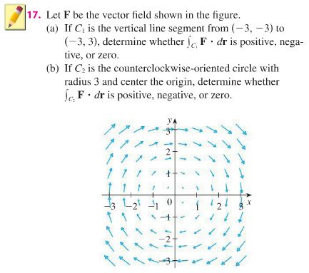
Th: 16.1: 1, 5, 11; 21, 23, 29, 31, 33;
comparison shopping (think of this as matching game, to see how to distinguish some feature of the formula by its graphical representation):
11-14: < x,-y>, <y, x - y>, <y, y + 2>, <cos(x+y), x> ;
15-18, <1, 2, 3>, <1, 2, z>, <x, y, 3>, <x, y, z> ;
29-32: x²+y², x(x+y), (x+y)², sin(x²+y²)^1/2;
19*; just try the template for this problem, no need to submit, or just read the worksheet and then the result, with bonus problem 25 done as well.

MLRC 5:30 voluntary problem session for Test 3.
F: Quiz 7 answer key on line; check Blackboard grades;
Take home Test 3 out in class. READ TEST INSTRUCTION WEBPAGE FIRST. This is due back in one week in class on Friday if you are able to budget adequate time to complete it to your satisfaction by then, otherwise by the following Monday 25 April in class.

WEEK 13: Maple 15? not required. Make sure you have 4/4 for first two assignments.
M: handout on line integrals (ignore text discussion of "scalar" integrals with respect to dx, dy, dz separately);
16.2 ( ∫ f ds scalar line integrals): 2, 3, 11 [write vector eq of line, t = 0..1];
33, 36 [if radius 1, ans: <4.60,0.14,-0.44>, worksheet compares with centroid: obvious midpoint, also bonus: 33 solution].
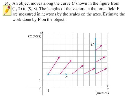
W: 16.2: handout with exercise on vector line integrals
( ∫ F · dr = ∫ F · (dr/dt) dt = ∫ F · T ds = ∫ F₁ dx +F₂ dy + ... ; always use vector notation!):
7 [ ∫_C <x+2y, x²> · <dx, dy>], 15, 17, [read: 27 Maple template for vector line integrals], 32, 39;
45, 51 (notice projection along line constant on each line segment, so can multiply it by the length, add two separate results);
scalar line int: 48;
inverse square force line integral example from 16.3 example 1.
Th: handout on "antidifferentiation" in multivariable calculus: potential function for conservative vector field;
16.3: 3, 7, 11 (b: find potential function and take difference, or do straight line segment line integral), 15 (potential function); 23, 25, 33, 35.
Optional note: the final section of 16.3 on conservation of energy is really important for physical applications but not required in this course. Enough said.
F: hand i Test 3 if you are satisfied with your completion;
16.4 (Green's theorem): 3, 7, 9, 17, "WA:501"
[polar coord problem not in WebAssign: 18, convert double integral to polar coordinates; ans: 12 π];
[optional: the line integral technique for integrating areas of regions of the plane is cute but we just don't have time for it so you can ignore it.]

Fri: 8pm, Sat:2pm,8pm support your talented fellow students who in spite of all the academic crunch time pressures, are putting on a delightful show for you: The Villanova University Student Musical Theater performances of The Fantastics in St Mary's Theater.

WEEK 14: final due date for take home Test 3 Monday in class.
M: handout on divergence and curl, Gauss and Stokes versions of Green's Theorem;
handout on interpretation of circulation and flux densities for curl and div [.mw: visualize];
[magnetic field lines; electric field lines];
16.5 (curl, div): 1, 3, 9-11,
12 [easier to interpret vectorially if convert to "del, del dot, del cross" form],
13, 19 [a magnetic field has div H = 0, so H = curl A is a way of representing it in terms of a vector potential so that it automatically has zero divergence, see problem 38; a static electric field has curl E = 0 so a scalar potential E = - grad φ is relevant---the minus sign is another story!],
31 [but read 37, 38 and look at identities 23-29].
T[F]:
Optional 16.6-7: surface integrals for fun;
Optional 16.8-9: read lightly Stokes' Theorem, Gauss's law if you are interested, when you have time;
[example1: centroid of hemisphere, Gauss law example, wedge of cylinder 16.7.example3;
example2: parabola of revolution (Stewart16.7.23 expanded into Gauss/Stokes examples)].
W: CATS evaluations;
Review problem 15.3.39 for final exam;
Verify Green's theorem for F = <-x^2 y,x y^2> (or Gauss-Green's theorem for G = <x y^2, x^2 y> ) and the circle of radius 2 centered at (2,0) in three ways: Cartesian, x independent; Cartesian, y independent; polar, θ independent. [pdf, mw]
Th: Test 3 answer key online:
archived final exam online: cylindrical and spherical coordinates, line integrals, Green's Theorem verification, curl and divergence, potential functions.

F: MLRC problem session. 4:00.

Final Exams: Saturday April 30 10:45--1:15, then following Friday May 5 2:30 - 5:00; you may exchange dates with permission.

∞ scroll up for current day

MAPLE HW files:
maple13.mw due: Week 6
maple14.mw due: Week 10
maple15.mw due: Week 12? nah!

*MAPLE homework log and instructions [asterisk "*" marked homework problems]

Test 1: Week 5: ; MLRC 5:30 problem session .
Test 2: Week 9-10: ; MLRC 5:30 problem session .
Test 3: WEEK 13: Take home out ; in ; MLRC problem session

FINAL EXAM: MWF 10:30 Sat Apr 30 10:45--1:15; MWF 12:30 Fri May 6 2:30 - 5:00; (switching days allowed but notify bob)

Graphing Calculator / Maple Checking ALLOWED FOR ALL QUIZZES/EXAMS

25-jan-2016 [course homepage]
[log from last time taught with Stewart Calculus 7e]

does anyone ever scroll down to the end?
careful explanation pdf