2 mass spring system worksheets and pdf notes
[by bob jantzen]

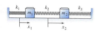
The figure shows 2 masses and 3 springs.
Setting k₃ = 0 yields the 2 spring system in this figure (no force exerted on second mass from the right).

Equations of motion setup: figure8curveset.pdf

2 springs (set k₃=0)

• 2mass2spring.pdf solved for general parameters
   
• 2mass2springperiodic.mw some periodic solution examples
  [2mass2springperiodic.pdf some hand written solutions, same coefficient matrix]
  (k₁, k₂) = (4,2),  (m₁, m₂) = (2,1)
  coefficient matrix: <<-3,1>,<2,-2>>, eigenfrequencies 1, 2
   
• 2mass2springaperiodic.mw some nonperiodic solution examples
  [2mass2springaperiodic.pdf some hand written solutions]
  (k₁, k₂) = (3,2),  (m₁, m₂) = (1,1)
  Same coefficient matrix: <<-5|2>,<2|-2>>, eigenfrequencies 1, sqrt(6)
   
• 2mass2springgravityex.pdf, 2mass2springgravityex_soln.pdf, 2mass2springgravityex.mw [constant gravity]
  [sinusoidal driven case, same matrix: 2mass2springex0.pdf]
  (k₁, k₂) = (3,2),  (m₁, m₂) = (1,1)
  Same coefficient matrix: <<-5|2>,<2|-2>>, eigenfrequencies 1, sqrt(6)
  
• 2mass2spring-triplefigure8.mw
  (k₁, k₂) = (1,4/3),  (m₁, m₂) = (3,4)
  coefficient matrix: 1/9 <<-7|4>,<3|-3>>, eigenfrequencies 1/3, 1; sinusoidal driving frequency 1/2;
  periods ( 6 π, 2 π, 4 π), common period 12 π; makes triple figure 8 (3 loops);
  homogeneous problem video: 2mass2springphaseplanevideo-triplefigureeight.gif
   
• How to generate parameter values that give simple eigenfrequencies: 2mass-springsystemtoyproblems.mw
  
  
• EPC4, example 7.5.1:
  (k₁, k₂) = (100,50),  (m₁, m₂) = (2,1)
  coefficient matrix: 25 <<-3|1>,<2|-2>>, eigenfrequencies 5, 10;
  periods ( 2 π/10, 2 π/5), common period 2 π / 5; 
      see above rescaled matrix (multiplied by a perfect square integer suggesting other variations)
  
• tuned mass dampers EPC4 7.5.14
  [adjusting the smaller second mass to stop the first mass from oscillating]
  

3 springs

• 2mass3spring.pdf solved for general parameters [2mass3spring.mw,]
• [2mass3spring-equal.pdf an example with equal masses and spring constants done by hand
  (k₁, k₂, k₃) = (1,1,1),  (m₁, m₂) = (1,1)
  coefficient matrix: <<-2,1>,<1,-2>>, eigenfrequencies 1, sqrt(2):]
  2mass3springequal.mw; equal masses and spring constants, nonperiodic motion
  [with reduction of order and damping-resonance bonus, highlighted graphics outside sections]; see also:
   reduction of order with exercise;  redorderexercise2.pdf;
   redorderwithoutredexercise3.pdf  [redorderexercise.mw]
        [Ignore previous version, yesterday only: redorderwithoutredexercise2.pdf]
  
   
• in class exercise:  driven 3 spring, 2 mass system, easy numbers, resonance
  (k₁, k₂, k₃) = (1,2,2),  (m₁, m₂) = (1,2)
     coefficient matrix:  <<-3,2>,<1,-2>>, eigenfrequencies 1, 2:
  epc4-7-5-3_9-brief.mw unequal masses and spring constants, periodic motion [with reduction of order and damping-resonance bonus]
  ep3_7-4_3-9.pdf
   
• in class exercise:  ep3_7-4-11.htm
  (k₁, k₂, k₃) = (32,8,32),  (m₁, m₂) = (1,2/3)
     coefficient matrix:  <<-40,8>,<12,-60>>, eigenfrequencies 6, 8
  (divide K matrix by 4 to reduce to 3,4: (k₁, k₂, k₃) = (8,2,8), <<-10,2>,<3,-15>>):
  unequal masses and spring constants, periodic motion
  
  
• explore3oscillationmodes.mw
  3 cosine modes explored: rational frequency ratio, irrational frequency ratio cases illustrated; convex hull of boundary points gives boundary of region of plane containing 3 oscillations
  
• 2mass-3spring-figure8curves.mw equal masses and unequal spring constants, periodic motion [with reduction of order and damping-resonance bonus]
  (k₁, k₂, k₃) = (1,3/2,1),  (m₁, m₂) = (1,1)
  coefficient matrix: <<-5/2|3/2>,<3/2|-5/2>>, eigenfrequencies 1, 2; driving frequency 3:
  see also desysdesys2x2order2ex.mw.
  Finally movies (2012-12) with adjustable initial conditions and driving amplitude and frequency!
       figure8curve.mw [jpg movie of 2 mass positions versus time, corresponding phase plane plot of the 3 independent modes:
      2 natural modes plus a response mode to a driving frequency]
      [in class exercise: drivenDEsystemExercise.pdf,
       solution: figure8curve12.pdf = figure8curve1.pdf + figure8curve2.pdf hom + nonhom deqs
       plot: figure8curvemodesplot.mw, figure8curvemodesplot.pdf ]
  hand: undriven figure8curve1.pdf, driven figure8curve2.pdf  F = <0,50 cos(3 t)> in x'' = A x + M^-1 F, where M is the mass matrix.
  More reduction of order, damping: figure8curve-reduction.mw
  
  Integer frequency toy problems:
  
• (k₁, k₂, k₃) = (6,4,6),  (m₁, m₂) = (1,1) : coefficient matrix: <<-10|6>,<6|-10>>, eigenfrequencies: 2,4
  B = <<1,1>|<-1,1>> [divide matrix by 4 to get eigenfrequencies 1,2]
• (k₁, k₂, k₃) = (6,2,3),  (m₁, m₂) = (1,1) : coefficient matrix: <<-8|2>,<2|-5>>, eigenfrequencies: 2,3
  B = <<1,2>|<-2,1>> [11S]
• (k₁, k₂, k₃) = (8,2,8),  (m₁, m₂) = (1,2/3) : coefficient matrix: <<-10|2>,<3|-15>>, eigenfrequencies: 3,4
  B = <<2,1>|<-1,3>> [12F]
• (k₁, k₂, k₃) = (4/9,2/9,0),  (m₁, m₂) = (2,1) : coefficient matrix: <<-3/9|1/9>,<2/9|-2/9>>, eigenfrequencies: 1/3,2/3
  B = <<1,2>|<-1,1>> [15F]
• (k₁, k₂, k₃) = (3/9,4/9,0),  (m₁, m₂) = (1,4/3) : coefficient matrix: <<-7/9|4/9>,<4/9|-4/9>>, eigenfrequencies: 1/3,1
  B = <<2,3>|<-2,1>> [13F]

N springs

• N = 5 and N ≥ 2: The special case of equal masses and spring constants between two walls, coded for any N but demonstrated for N = 5
   5mass6springsystems.mw [5mass6springvideo.gif]
  This can be solved exactly since the coefficient matrix in the equations of motion is a symmetric tridiagonal Toeflitz (band) matrix.

multistory building sideways motion in earthquake analysis

• earthquakelinks.htm [7 mass, 7 spring problem modeling a 7 story building, Edwards and Penny Application 7-4]
  The coefficient matrix differs from a tridiagonal Toeflitz (band) matrix (as in the previous case) by its last diagonal entry (last floor has no floor above it), so that no simple exact formula exists for the eigenvalues so one is forced to numerical results.
• a related idea involves damping out the swaying motion of tall buildings with dynamic damping; instead of horizontal forces applied to the base of the building, winds apply lateral forces to the side of the building.

understanding eigenvectors

• Watch the MIT Eigenvector 4 minute video [there are 6 frames which then repeat, so stop when you see it beginning again---from their LinAlg course; no longer available]; see the 6 possibilities of the video in this Maple DEPlot directionfield phaseplot template with Maple directionfield plots of each associated linear vector field A x allowing local visualization of the action of matrix multiplication by the matrix A.  [MIT & FLASH gone!]
   
• Duke University on-line linear system interactive Java applets [Java GONE!]
  [The most popular browsers no longer support Java;
  BUT now Maple can substitute this app with a worksheet described  below.]
  Then play an interactive computer game with the Duke U applet lining up the vectors [red is x, blue is A x, click on matrix entries to change, click on tip of red vector  x and drag around an approximate circle to see corresponding blue vector A x]; try first with the default values, then try for a₁₁=0, a₁₂=1, a₂₁=1, a₂₂=0, then try for the matrices of Edwards and Penney Edwards and Penney DE and LinAlg: 6.1: 1,2. See if you can guess the eigenvector directions and the corresponding eigenvalues (all integer triangles locating the vectors and integer eigenvalues); write down a simple representative eigenvector (with the smallest integer components, say) and its eigenvalue that you can read off from the applet as explained within the introductory webpage.
  
• Here is a Maple worksheet which duplicates the Duke University applet (as best it can) using the MIT matrices of the Maple worksheet in the first item, mouse dragging of the tip of the input vector to line it up with the output vector and then scale it up to match the grid so that one can easily read off/estimate the multiplier (eigenvalue!) for the output vector along an eigendirection when the input and output vectors line up:  exploreeigendrag.htm.
  
  
• Here is a cute interactive slider applet showing the solutions of a coupled pair of linear constant coefficient differential equations which could easily be duplicated in Maple with the Explore command:
  https://mattlane.us/stories/gaming-relationships-linear/