MAT2705 20F homework and daily class log

Jump to current date! [where @ is located]

Daily lectures and your homework will appear here each day as it is assigned, including some PDF and/or Maple problem solution files or PDF notes, with occasional links to some MAPLE worksheets when helpful to illustrate some points where technology can be useful. [There are 56 class days in the semester, 4 each normal week, numbered consecutively below and  labeled by the (first initial of the) day of the week. Friday will usually be the quiz day. Monday quiz makeup day.]

It is your responsibility to check homework here since not all homework exercises are online. (Put a favorite in your browser to the class homepage.) You are responsible for any hyperlinked material here as well as requesting any handouts or returned tests or quizzes from classes you missed. Homework is understood to be done by the  next class meeting (unless that class is a test, in which case the homework is due the following class meeting), but the online deadline will be stated as midnight of the due day so that you have time in class or after to ask questions that you did not submit via the Ask the Instructor online tool. You may correct submitted homeworailyk after the deadline without having to request an extension.
[[Homework problems surrounded by double square brackets [[...]] are not in the online homework system but are important to do.]]

Read:  HOMEWORK ADVICE;       ZOOM CLASSROOM/OFFICE HOUR INFO
quiz, test BlackBoard access/submission

1. M:  (August 17)
   DURING CLASS:
   Lecture Notes 1.1a: Differential Equations: how to state them and "check" a solution;
   summary handout: odecheck.pdf
   
   New to Maple 3 minute video
   
   AFTER CLASS (THIS IS THE HOMEWORK):
   1) Log on to My Nova, choose the Class Schedule with Photos, view fellow students.
   2) Go to BlackBoard and look at the class portal and Grade book for our course: you will find all your Quiz, Test and Maple grades here during the semester once there is something to post. Everything we do except for quizzes, tests and grades will take place through our course website.
   3) Download Maple 2020 for Windows or Mac if you haven't already done so and install it on your laptop when you get a chance (it takes about 15 minutes). If you have any trouble, email me with an explanation of the errors.
   You are expected to be able to use Maple on your laptop when needed. We will develop the experience as we go. No previous experience is assumed.
   4) Enter the e-text MyLab Math portal if you have not already done so!
       registration codes: 004: jantzen48548, 005: jantzen35255 [click codes for detailed instructions]
   5) Homework Problems: 1.1: 3, 5, 13, 33 online.
   [memorize!: "A is proportional to B" means "A = k B" where k is some constant, independent of A and B]
   (short list so you can check out our class website and read about the course rules, advice, bob FAQ, etc, respond with your email).
   It is important that you read the section in the book from which homework problems have been selected before attempting them.
   Optional: get acquainted with Maple clickable calculus DE entry and "odetest" for problems 3,5,13 [even 33!]
   
   Proportionality statements must be converted to equalities with a constant of proportionality introduced:
   y is proportional to x:  y ∝ x  means y = k x . [y is a multiple of x]
   y is inversely proportional to x:  y ∝ 1/x  means y = k/x .
   y is inversely proportional to the square of x:  y ∝ 1/x²  means y = k/x²
   6) By the end of the week, reply to my welcome e-mail from your OFFICIAL Villanova e-mail account (which identifies you with your full name), telling about your last math courses, your comfort level with graphing calculators and computers and math itself, [for sophomores only] how much experience you have with Maple (and Mathcad if appropriate) so far, why you chose your major, etc, anything you want to let me know about yourself that will give me more of an idea about you as a person. [For example, I like to do humorous sketching. and cooking.] Tell me what your previous math course was named (if at VU: Mat1500 = Calc 1, Mat1505 = Calc 2, Mat2500 = Calc3).
   [In ALL email to me, include the string "mat2705" somewhere in the subject heading if you want me to read it quickly. I filter my email.]
   
   
2. T: Lecture Notes 1.1b: Differential Equations: initial conditions
   1:1: 8, 23 [see Maple plot (execute worksheet by clicking on the !!! icon on the toolbar)];
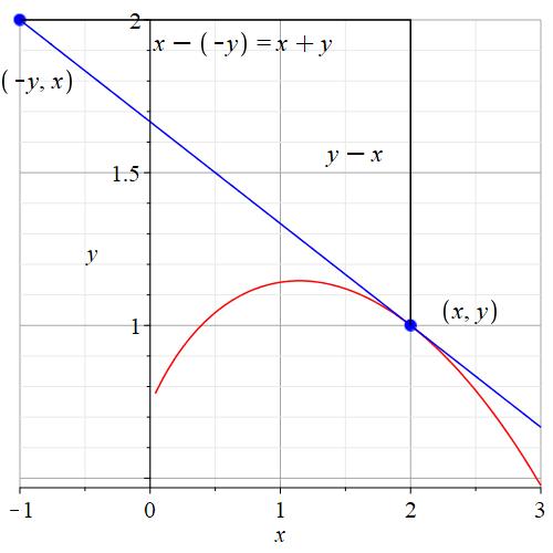
   formulating DEs: 27 [approach like 29, make a generic diagram like this one to calculat the slope of the tangent line and set it equal to the derivative .mw],
   [[29. Hint: recall perp lines have slopes which are negative reciprocals, the normal line is perpendicular to the tangent line and passes through the same point on the curve; make a diagram of the given point (0,1), a "generic" function graph curve whose normal at a point (x,y) on the curve passes through (0,1), and draw in the connecting normal line segment between these two points and the perpendicular tangent line, then compute the slope of the normal line from the two points, and then from the negative reciprocal of the derivative value, finally equate the two to get the DE: mw ]],
   31, 35, 43;
   on-line handout: initial data: what's the deal?
   
   Is your dorm abbreviation missing from bob's dorm list?
   
   
3. W:  read the handout: algebra/calc background sheet [online only: more rules of algebra NOT!];
   Lecture Notes 1.2: First order DEs independent of the unknown [some redundancy with previous lecture, plus two word problems];
    [lunar landing example: mw] [Swimmer problem example: mw]
   1.2 (antiderivatives as DEs): 1, 5, 15,
   21 [Hint: write piecewise linear function from graph: v₁(t) for first expression, v₂(t) for second expression, solve first IVP for x₁(0) = 0, second IVP for x₂(4) = x₁(4); example: pdf, mw],
   25 (like lunar landing problem, see example), 35,
   41 (mw: short, long)
   [[43 (pdf) [convert to appropriate units!]].
   
   Nongraded Blackboard Quiz 0 due today by 11:59pm. Does anyone not have access to a printer?
   remind bob to demonstrate quiz upload
   
   
4. F: Quiz 1 (read Test/Quiz rules; submission instructions): due Sat 11:59pm, start in class;
   if time, more discussion of 1.2 river crossing problem;
   Lecture Notes 1.3: First order DEs; Direction (= slope) fields and complications
   [directionfields.mw] [ode1-complications.mw]
   1.3 direction fields: 3, 11, 15;
   [[optional: 1.3: 3: for fun hand draw in all the curves with a pencil on the full page paper printout: projectable image; bob's  attempt]
     try the Maple template for 5]]
   
   WEEK 2:
5. M: Quiz one answer key;
   Lecture Notes 1.4a: Separable first order DEs
   [ example 1: implicit soln,  other complications visualized].
   1.4 (separable DEs): 1, 4, 9 (see mw!), 25, 27, 29.
   
   Office hours; Course "Syllabus" now online; Final Exam dates
   HW "due date" = Dec 6 to allow resubmission of answers until you get it right
   but HW "due" the day after it is assigned to keep on track.
   
   
6. T: Lecture Notes 1.4b: Separable first order DEs
   handout on exponential behavior/ characteristic time       [how to plot?] [cooking roast in oven remarks]
   [read this worksheet explicit plot example, execute worksheet first with !!! icon on toolbar];
   1.3.3 online;
   1.4: 33, 35, 41,
   45 (if your cell phone were waterproof: "Can you hear me now?" attentuation of signal--characteristic length),
   49.
   
   
7. W: 1.4: 69,
   [[65. CSI problem  (Newton's law of cooling) same as worked problem but at end we want to find a previous time instead of a subsequent time]].
   Maple play to help familiarize you with using it. Split screen between my projected Maple and your local Maple so you can try it out.
   We take a breather to catch up.
   Hyperbolic functions are important in DEs! [wiki]
   
   Optional: after you solve this problem yourself, consult both [pdf, .mw];
     please read Maple worksheet to see the power of mathematics to solve all such problems at once;
     please read the PDF to see how to convert the word problem line by line to a mathematical problem].
    If curious: revisit the river crossing problem and the oven heating problem.
   
   Bonus discussion: average value of velocity profile: river crossing problem
   [please read this Maple worksheet to see the power of mathematics to solve all such problems at once]
   
   
8. F: Quiz 2 (separable DEs, see Quiz 2 in archive);
   Lecture Notes 1.5a: Linear first order DEs
   online handout: recipe for first order linear DE [plot] [mw exploration]
   1.5: 2, 5, 8, 21, 24;
   *[check at least one of these problems, both the general solution and the initial value problem solution with the dsolve template].
   
   For future reference:
   > deq := y ' = x y      [space implies multiplication]
   > sol:=dsolve(deq, y(x))
   > solinit := dsolve({deq, y(0)=1}, y(x))
   [or enter DE plus IC separated by a comma, right click on output, choose Solve DE, for y(x), or Solve DE interactively;
   rightclick "Simplify, Simplify" or "Simplify, Symbolic" (with radicals) may be necessary to simplify the result]
   > y ' = x y , y(0)=1
   Use function notation to change independent variable:
   > y '(t) = t y(t) , y(0) = 1
   
   class directory list (image only by email for privacy reasons);
   
   WEEK 3:
9. M: Lecture Notes 1.5b: Linear first order DEs:complications  [acc. funcs.: mw] [Khan] [slope field: mw]
   1.5: 15, 24, 27; 30;
   [[29: solutions defined by a definite integral. Use the fact that the derivative of the function defined by the integral is the integrand including all multiplicative factors ]];
   [[41 in class activity with breakout rooms if bob can make them work: epc4-1-5-41.htm ]]
   
   
10. T:  Lecture Notes 1.5c: Linear first order DEs: Mixing Problems [Maple template]
    [this mixing tank problem is an example of developing and solving a differential equation that models a physical situation (online handout); ];
    1.5 (ChE majors especially) Use Eq. 18 in the book or the boxed equation in the online handout:
    respectively constant, decreasing, increasing volumes: 33, 36, 37;
    constant volume lake application: 45;  [solution worksheets];
    we attempt another breakout session on problem 33 collaboration;
    optional extra questions interesting to answer: what is the final concentration? How does it compare to the initial concentration and the incoming concentration?
    
    Note: we are skipping 1.6: exact DE etc. These are less important, and Maple can solve these when needed anyway. A similar integrating factor technique works for exact equations but where the independent and dependent variables are on an equal footing.
    
    
11. W: 1.R (review): be prepared in class to classify the odd problems 1-35 as: separable, linear in y (as unknown), linear in x (as unknown), some combination of these three, or NOTA (none of the above, i.e., from skipped section 1.6), for example dy/dx = y/x is all three and can be solved in three different ways; don't solve them but (review problems are not online):
    [[ solve 25 [it can be done in two ways by expanding out the square on the RHS before integrating with integration constant C or by using a u-substitution as the book did with integration constant K; express K in terms of C as given in the book supplied answers by combining the two terms in the K solution [identity for expanding out (x+1)³ !] and then comparing with the C solution];
    solve 35 in two ways and compare the results---different constants enter your expressions, show how they agree]];
    for another word problem example, see this (both linear and separable; similar to late stages of logistic behavior next section)
    
    
    
12. F: Quiz 3 (linear DE see quiz 3 in archive); check your graded Quiz 2 in BlackBoard;
    Lecture Notes 2.1a: First order DEs: Logistic Equation
    handout on solution of logistic DEQ [Maple: characteristic time /shape,  directionfield,  integral formula, 24];
    2.1 (logistic DE): 5 (resolve the DE this one time following the steps in the Lecture Notes),
    6 (reverse S curve, choose a horizontal window to show full S curve based on plus/minus 5 times characteristic time,
    answer: > dsolve({x'(t) =3 x(t) (x(t)-5), x(0)=2},x(t)) (copy and paste into the input line, rightclick choose RHS, then from the CSM choose Plotbuilder, choose horizontal window based on characteristic time, make sure you then see the S-curve without wasting too much window where nothing is happening);
    17 (see Maple worksheet for setup problem 15);
    21 (initial value of population and its derivative given instead of population at two times, need to set k and P(0) with two conditions),
    23 [Note dx/dt = 0.004 x (200-x) so k = 0.004, M=200 for logistic curve solution formula],
    29.
    
    WEEK 4[-1]:
    M: Labor Day
13. T: Lecture Notes 2.1b: First order DEs: More models, Separable: f(y)
    2.1 (other population models):
    handout on DE's that don't involve the ind var explicitly;
    11 ["inversely propto sqrt": use β = k₁/P^(1/2), δ = k₂/P^(1/2) in eq.(1), these are fractional birth/death rates;
    leads to P' ~ P^(1/2) soln],
    13 [P' ~ P^2 example],
    [[30, 31 [ans: find β_o = 0.3 from condition dP/dt(0) = 3x10^5 using the DE at t =0, then use solution α=0.3915 from second condition (solve this yourself or at least check numerically that it satisfies the 6 month condition) to find the limiting population as t goes to infinity (i.e., neglect decaying exponential)]].
    39 [oscillating growth].
    
    
14. W: Lecture Notes 2.3: First order DEs: acceleration models
    2.3 (acceleration-velocity models: air resistance):
     air resistance handout (example of a piecewise defined DE and solution and the importance of dimensionless variables);
    [optional reading to show what is possible: comparison of linear, quadratic cases; numerical solution for any power];
    2;3: 1, 3,
    9 [remember weight is mg, so mg = 32000 lb determines mass m = 1000 in USA "slug" units, convert final speed to mph for interpretation!],
    17 [v > 0 falling slowing down to stop, plug in numbers],
    19 [constant thrust = reverse gravity!];
    [[optional reading: 22 this is the tanh case: v_terminal = 20.7 ft/s, t = 8 min 5 s].[soln, .mw]]]
    
    
15. F: Quiz 4 on population modeling, like HW problems;
    Lecture Notes 2.4: First order DEs: numerical DE solving (Euler)
    2.4 (Euler numerical solution): 1, 27 [this shows the Maple approach],  29 [naive approach]
    [[optional reading: example. problem 1 studied in detail showing the algorithm with euler-doc.mw, soln)]]
    
    
    WEEK 5[-1]: detour into linear algebra; Test 1 on first order DEs next weekend, starting in class Friday?
16. M: Lecture Notes 3.1: linear systems of equations: elimination, DEs;  [inconsistent 3x3 system; DEs lead to linear systems];
    why LinAlg with DE?; [maple dsolve and DEplot for 2x2 systems of DEQs];
    Read 3.1 on linear systems (review of high school topic solving 2 or 3 linear equations in 2 or 3 variables),
    do 3.1: 3, 5, 7; 9, 23, 25.
    
    Check  answer key for Quiz 4.
    
    
    
17. T: 3.2: Lecture Notes 3.2: matrices and row reduction "elmination";
    handout on RREF (Reduced Row Echelon Form, section 3.3) [see bob's examples 2, 3 using Maple];
    3.2: 1, 5, 7, 9; 11,13,15,
    (1, 5, 7 already Gaussian reduced, for rest do a few RREF by hand, then you may use step-by-step row ops with MAPLE or a calculator for the rest) ;
    [Matrices for doing some of tonight's homework with Maple preloaded];
    you must learn a technology method since this is insane to do by hand after the first few simple examples);
    23 [can your calculator handle this?]
    
    
    
18. W: 3.3: Lecture Notes 3.3: Row reduction solution of linear systems;
    handout on  solving linear systems example [.mw];
     we always want to do a full [Gauss-Jordan] reduction, not the partial Gauss elimination reduction also described by the textbook;
    the Matrix palette inserts a matrix of a given number of rows and columns;tab between entries;
    in breakout rooms of 2 open this Maple file and use the LinearSolveTutor and enter the matrix for the system 3.2.15 given there and reduce step by step, then solve the system (if possible), then switch positions and enter the matrix for the system 3.2.18 given there and repeat using instead the Reduction command template there;
    
    3.3: 1, 3, 9, 11, 14, 16, 17, 19, 23 (= 3.2.13), 29 (=3.2.19)
     Since the homework portal changes the matrices, I cannot preload them for you. But you can use this template to invoke the Tutors and the reduction and solving commands.
    
    
    
19. F: Test 1 on 1st order DEs in usual Quiz format due Sunday midnight:
    1 population modeling problem, 1 linear DE, 1 separable DE, so 2.5 days to do three homework problems well.
    Read Test Instructions; Remember bob is trusting you to observe our Villanova honor system.
    Lecture Notes 3.3: Balancing Chemical Reaction Application (short lecture);
    In class breakout room fun: Application: chemical reaction problem.
    (what can you find out on the web about interpreting this chemical reaction? chem site reaction balancer gives balanced reactions but no description, this one of our exercise turns out to be interesting).
    
    word of the day (semester really): can you say "homogeneous"? [online handout only]
    Get used to this word, it will be used the rest of the semester. It refers to any linear equation not containing any terms which do not have either the unknowns or any of their derivatives present, i.e., if in standard form with all the terms involving only the unknowns on the left hand side of the linear equation, the right hand side is ZERO. [nonhomogeneous means the RHS is nonzero]
    
    
    WEEK 6[-1]:
20. M: Lecture Notes 3.4: Matrix operations [finally matrix multiplication: handout];
    in progress:
    3.4: 1, 5, 7, 9, 13, 15, 17, 19; [[read: 27, check with Maple: 43]];
    Matrix algebra is easy in Maple [see here for how to do Matrix stuff in Maple].
    
    
    
21. T: Lecture Notes 3.5: Matrix inverses; [Maple inverse template: mw]; [2x2 inverse! mw, pdf]
    3.5: 1, 5, 7, 9, use Maple to do row reductions: 11, 19,
    23 [Maple template; this is a way of solving 3 linear systems with same coefficient matrix simultaneously, as in the alternative derivation of the matrix inverse];
    30.
     
     Matrix multiplication and matrix inverse, determinant, transpose [or right-click and use Standard Operations menu]
     > A B [note space between symbols to imply multiplication]
     > A^-1
     > |A|   [absolute value sign gives determinant, or just right click]
    Memorize: . Switch diagonal entries. Change sign off-diagonal entries. Divide by determinant.
    Always check inverse in Maple if you are not good at remembering this.
    
    
    
22. W: 3.6: Lecture Notes 3.6: Matrix determinants;
    [forget cofactors, forget Cramer's rule (except remember what it is when old-fashioned texts refer to it), use Maple instead];
    optional on-line handout: determinants and area etc ;
    [optional: why the transpose? (to combine vectors we arrange them into rows of matrix, the transpose maps columns to rows, rows back to columns)];
    Read explanation of why we need determinants; 
    3.6: (determinants abbreviated: forget about minors, cofactors, only need row reduction evaluation to understand)
    7, 9, 10,  13, 15, 17, 25, 29.
    [[7*use this example to record your Gaussian elimination steps in reducing this to triangular form and check det value against your result]].
    
    Optional. Explanation of why determinants are important for measuring area and volume etc in higher dimensions. [Calc 3 stuff]
    
    
23. F: Quiz 5 row reduction and solving a linear system;
    Lecture Notes 4.1: Linear independence;
    R^n spaces and linear independence of a set of vectors [motivating example];
    now we look at linear system coefficient matrices A as collections of columns A = < C₁| ... |C_n >,
    matrix multiplication on the right by a column of coefficients as taking linear combinations of those columns,
    A x = x₁ C₁ + ... + x_n C_n
    and solving homogeneous linear systems of equations  A x = 0  as looking for linear relationships among those columns (nonzero solns=linear rels) ;
    4.1: 5, 7; 13; 15, 17; 19, 23; 29, 31, 33
    [use technology in both 1) evaluating the determinant  and 2) contexyt sensitive menu for the ReducedRowEchelonForm needed for these problems];
    
    hand out on the interpretation of solving linear homogeneous systems of equations: A x = 0
      [optional read: visualize the vectors from the handout].
    
    WEEK 7[-1]:
24. M: Lecture Notes 4.2: Vector spaces and subspaces;
    study the handout on solving linear systems revisited [remember the original one: solving linear systems example];
    [note only a set of vectors x resulting from the solution of a linear homogeneous condition A x = 0 can be a subspace of a vector space; interpretation: lines, planes, ..., hyperplanes through the origin];
    4.2: 1, 3, 7, 11; 15, 21.
    
    
25. T: Lecture Notes 4.3: Span of a set of vectors;
    so far: linear independence (A x = 0), express a vector as a linear combination (A x = b)
     [or does b belong to a linear relationship with the columns of A?];
    4.3 (span of a set of vectors):  1, 3, 5, 7; 9, 13; 17, 21.
    
    Test 1 answer key is online; read  test1-20f-remarks.htm.  
    For those curious about what the value of a determinant means read this.
    
    
    
26. W:  Lecture Notes 4.4: Bases;
    handout on linear combinations, forwards and backwards [maple to visualize]
    4.4: 1, 3, 5, 7;
    9 [this is already reduced, find solution as in class example, pull apart to find coefficient vectors of parameters, repeat for next 4 problems reducing first],
    13; 15, 17, 25 [use technology for all HW row reductions and determinants (but 2x2 dets are easy by hand!)].
    
    
27. F:  Quiz 6 on solving linear systems and linear independence;
    handout on nonstandard coordinates on R² and R³ [goal: understand the jargon and how things work];
    0) bob tries to draw this out on the white board, explaining how it works.
    Then in the breakout rooms, you do the following each separately, but discussing and critiquing each other's work (hold it up to the screen, enlarged for the person trying to share their work in speaker view!).
    1) Using the completed first page coordinate handout made for that new basis {[2,1],[1,3]} of the plane just explained by bob, graphically find the new coordinates of the point [4,7] reading off the grid. Then find the old coordinates for the point whose new coordinates are  [2,2]. Your graphical read outs can be confirmed by the corresponding matrix multiplications if there is disagreement.
    2) Next practice on the blank grid [ .mw, .pdf] you printed out in advance with b₁= <3,-1>,  b₂= <2,2> . Draw these arrows at the origin, and then replicate then tip to tail along the new coordinate axes, marking off the new tickmarks and reproduce the grid corresponding to  -2..2 in the new coordinate tickmarks. What are the new coords of the point (position vector!)  <-2,6>? What point (position vector!) has new coords <2,-1>?] .
    3) Next we change to new basis vectors and using the above handout as a guide, complete the blank worksheet printed out in advance, similarly drawing its new basis vectors and axes with tickmarks and the grid, etc. Use a ruler and sharp pencil,to make a new -2..2,-2..2 coordinate grid associated with the new basis vectors {[1,1],[-2,1]} and graphically represent the point [x₁,x₂] = [-5,1] and find its new coordinates  [y₁,y₂] using the grid. Similarly read off the old coordinates [x₁,x₂] of the point whose new coordinates are [y₁,y₂] = [-2,-1]. Confirm that these agree with the corresponding matrix calculations. Put your name on it, scan it to lastname-firstname-quiznot.pdf and email it to me by next class with the filename in the subject header next class: 
    Subject: mat2705: LastName-FirstName-Quiznot.pdf.  [not for credit]
    
    solution:   completed worksheet [Maple version of the example]
    
    not Fall break week follows week 7! not this year!
    
    
    WEEK 8[-1]:
28. M: 4.7  Lecture Notes 4.7: Vector spaces of functions;
    bridge to vector spaces whose elements are functions.
    
    handout summarizing linear vocabulary for sets of vectors;  
    [optional on-line handout: linear system vocabulary for linear systems of equations ]
    Part 2 of course begins: transition back to DEs:
    read the 4.7 subsection (p.279) on function spaces and then examples 3, 6, 7, 8;
    if you are curious, example 5 illustrates the partial fraction decomposition needed in engineering integration;
    read the worksheet on the vector space of (at most) quadratic functions [quadratics.mw, pdf];
    4.7: 9. 11, 14 ( c₁ f₁(x)+  c₂ f₂(x) = 0, set x = 0 to get one condition on the two coefficients, set x = 1 to get a second, then solve 2x2 system),
    15 [Hint: solve c₁(1 + x) + c₂(1 - x) + c₃(1 - x²) = 0, for unknowns c₁,c₂,c₃; are there nonzero solutions? if not, these are linearly independent polynomials, in terms of which any quadratic expression in x can be written; note that any two (nonzero!) functions of x that are not proportional are automatically linearly independent],
    18 [same approach].
    
    Reminder: vectors are identified with column matrices!
    Optional Reading: Why do we care about linear coordinate grids in the plane?
    
    
29. T: Lecture Notes 5.1a: 2nd order linear DEs: an intro;
    read 5.1 up to the subsection on linear independence;
    Memorize: y ' = k y  < -- > y = C e ^{k x}
       y '' + ω² y  = 0 < -- >  y = C₁ cos(ω x) + C₂ sin(ω x)
    ["omega" = ω is the angular frequency "radians per time unit" as opposed to just "frequency" f = ω/(2π ) or "revolutions or cycles per time unit" as in physics, but in our class we will just say "frequency" for ω, assumed to be expressed in radians per time unit or converted to revolutions per time unit as convenient;
    see also damped harmonic oscillators and RLC circuits, and Hertz, not just a rental car company but "cycles per second"]
    5.1: 1, 3, 9, 11, 17.
    
    
30. W: Lecture Notes 5.1b: constant coefficient 2nd order linear homogeneous DEs;
     handout on sinusoidal example; repeated root plot;
     5.1[from linearly independent subsection]: 33, 35, 39,
    [[49 find the IVP solution for y, set y ' = 0 and solve exactly for x, backsubstitute into y and simplify using rules of exponents
    check your IVP solution for this curve in Figure 5.1.6; does the back of book answer y = 16/7 in decimal approximation agree with the figure?]].
    
    For those of you who did not submit the quiznot, you can try problems from older test 2 exams, which all have answer keys. But you have to do it yourself first, then look at the answer key or it will not be of much use.
    
    
31. F: No Quiz. Test 2 on chapters 3,4.
    read handout on complex arithmetic, exponentials [Maple commands; the complex number i is uppercase I  in Maple];
    
    
    WEEK 9[-1]:
32. M: Lecture Notes 5.2: The Wronskian and higher order constant coefficient 2nd order linear DEs;
    online handout: wronskian and higher order constant coefficient linear homogeneous DEs; [Maple Wronskian]
    5.2: 1, 7, [[11]],  13, 17, 23.
    
    
33. T: Lecture Notes 5.3a: higher order constant coefficient linear homogeneous DEs and complex exponentials;
    [sinusoidaldecay.mw]  [Maple Wronskian part 2]
    complex root handouts:
    1) general amplitude and phase shift of sinusoidal functions;
    2) 4 quadrant amplitude-phase shift examples: sinusoidquadrantex.mw, [[exp-cos-sin.mw]];
    3) exponentially modulated sinusoidal functions 
    4) summary handout: sinusoidal decay DE example with complex basis
    
    5.3: 1, 5, 9, 17, 21, 23, 33;
    [[23 exanple expressed in phase-shifted cosine form, another example: 25]];
    
    [ignore instructions to factor by hand or polynomial long divide: use technology for all factoring (bad roots!)].
    
    
34. W:  Lecture Notes 5.3b: higher order constant coefficient linear homogeneous DEs: repeated roots;
     [Maple Wronskian part 3] [phasor?]
    5.3 (higher order DEs):
    13, 33(oops), 41, 48 [[optional repeated complex roots: 16, 20]]
    [[IMPORTANT: For the decaying sinusoidal function: y(t) = exp(-2 t) (-3 cos(5 t)+4 sin(5 t)),
    a) evaluate numerically the frequency ω, the period T, the characteristic time τ, the ratio 5 τ /T, the initial amplitude and the phase shift in radians, degrees and cycles. Identify the two envelope functions. Make a plot in the natural decay window of the function and its envelope.
    b) Evaluate the initial data or state vector for this function. What are the complex roots which give rise to this solution of a linear homogeneous DE (r = -1/τ  plus/minus i ω ) and therefore what is the quadratic characteristic equation and the corresponding DE for which this is a solution?]]
    
    repeated root cases: 5.3: 11, 25 (the hw portal has very few repeated root problems!)
    
    
35. F: Quiz 7 (complex root pair DE like this quiz);
    Lecture Notes 5.4: Linear homogeneous 2nd order DEQ with constant positive coefficients (damped harmonic oscillators);
    handout on linear homogeneous 2nd order DEQ with constant positive coefficients (damped harmonic oscillator)
    5.4: 3  [use meter units!], 13 (maximum displacement), [[damped oscillations: 14]] , 15, 17, 19
     [[ read 23, pdf; this is a useful application problem]].
    
    
    WEEK 10[-1]:
36. M: Lecture Notes 5.5: NON-homogeneous 2nd order DEQ with constant coefficients; [mw];
    handout on driven (nonhomogeneous) constant coeff linear DEs; [final exercise on this handout sheet: pdf solution];
    5.5: 1, 3, 4, 8, 10, 13, 17, 33, 37 (pdf) [not easy for me either!]
    [not many of the book RHS driving functions are physically interesting here;
    we will not cover "variation of parameters"; the book presentation of the method of undetermined coefficients is a recipe with little justification (educated guess), instead the handout shows exactly how and why one gets the particular solutions up to these coefficients].
    
    
    
37. T: Lecture Notes 5.6a: Driven damped harmonic oscillators;
    handout on damped harmonic oscillator driven by sinusoidal driving function [1 sheet printable version];
    [in class example.mw pdf: resonance calculation side by side], maple resonance plots: general, specific];
    Note the HW portal wants the phase shift δ chosen between 0 and 2 π:
    5.6: 1, 3, 11, 13, 17 (template for final 3 problems, the HW portal wants the hase-shifted the cosine form for both steady state and transient in 11, 13 with 3 decimal place parameter values);
    
    Wiki: driven harmonic motion, amplitude plots: they introduce ζ = 1/(2Q)].
    
    
38. W: 5.6: Lecture Notes 5.6b: Driven damped harmonic oscillators: special cases;
    handout on beating and resonance [mw, with optional beating plot problem];
    Online HW catchup day. Don't let these go unfinished. Get bob's help.
    optional 5.6: 1 [worksheet rewrites this as a product of sines using the cosine difference formula:
    cos(A) - cos(B) = {-2 sin((A-B)/2)} sin((A+B)/2), the expression in {} is the sinusoidal amplitude envelope function [and its period is T = 2(2 π)/(A-B)], look at the plot of x and +/- this amplitude function (the envelope) together in this beating example worksheet, then do as explained here, repeat for the HW problem described in this link as well as at the end of this same beating example worksheet (be sure to plot one full period of the envelope function to see exactly 2 beats],
    
    We will watch the 4 minute Google linked video of resonance NOT! (but see the engineering explanation linked PDF for the detailed explanation):
    [Tacoma Narrows Bridge collapse (resonance NOT!): Wikipedia; Google (You-Tube video)];
    a real resonance bridge problem occurred more recently: the Millenium Bridge resonance (5 minutes).
    

    We will watch a 9 minute YouTube video massdampers.htm that shows a physical problem using the mathematics we will work up to by the end
    of the semester, two coupled damped oscillators, which is a simple model for realistic damping of the swaying motion of tall skyscrapers.

     
    Read 5.6.23 (earthquake!): consistent units: sec, ft, lbs; first evaluate Hookes' law constant, then find x''+10 x =  A₀ ω² sin(ω t), convert frequency to ω = 2 π /2.25 radians/s, set A₀  (=3in) = 1/4 ft. Solve. Find amplitude of response oscillation in inches.  [soln]
    
    Ignore this: EE/Physics majors if you are interested: RLC circuit application (floating point numbers!): RLC circuits [maple plots]
    
    
    
39. F: Quiz 8 like 18F:Quiz 8;
    Lecture Notes 6.1a: Eigenvectors and eigenvalues;
    Transition back to linear algebra:
    [In class watch bob use the Maple worksheet ExploreEigenDrag.mw to graphically determine the eigenvectors and eigenvalues of three 2x2 matrices. Recall old handout coupled system of DEQs and its directionfield [motivation: direction fields for Maple help visualize eigendirections of a 2x2 matrix]
    watch the MIT Eigenvector 4 minute video [requires IE browser because of Flash; there are 6 frames which then repeat, so stop when you see it beginning again---from their LinAlg course]; see the 6 possibilities of the video in this Maple worksheet DEPlot directionfield phaseplot template;
    then play a computer game with that Maple worksheet lining up the vectors [red is x, blue is A x, click on matrix entries to change, click on tip of red vector and drag around an approximate circle to see corresponding blue vector]; try first with the default values, then try for a₁₁=0, a₁₂=1, a₂₁=1, a₂₂=0, then try  for the matrices of 6.1: 1,2,7. See if you can guess the eigenvector directions and the corresponding eigenvalues (all integer triangles locating the vectors and integer eigenvalues)  for these matrices; write down a simple representative eigenvector (with the smallest integer components, say) and its eigenvalue that you can read off from the applet as explained within the introductory webpage to compare with your matrix calculations for these textbook HW problems . Then find them by the eigenvector process.
    
    6.1: 1, 2, 7 [1, 2, 7 mw]; 13;  Ignore polynomial division discussion, use technology for roots of polynomials!
    
    frequency: f or ω ?
    angular frequency ω is in radians/time but "ordinary" frequency is in cycles/time (number of multiples of one revolution of the circle): ω = 2 π f . Multiplying the frequency by 2 π radians converts it from a pure number of revolutions to radians per time unit. The reciprocal of the frequency f is just the period T = 1/f = 2 π / ω . We only need angular frequency in our course, but when we re-express such frequencies in Hz (cycles/sec) we are converting to the ordinary frequency for ease of interpretation, since radian units mean nothing to us.
    
    WEEK 11[-1]:
40. M: Lecture Notes 6.1b: Eigenvectors and eigenvalues: more (linear independence, complex eigenvectors);
    Maple 3x3 matrix eigenvector example handout [.pdf, real3x3 .mw; complex];
    6.1: 15, 19, 23 (upper triangular so diagonal values are eigenvalues!), (complex:) 29, 31 
    [do everything by hand for 2x2 matrices;
     for 3x3 or higher, go thru process: use Maple determinant: |A-λI| = 0 (right click on matrix, Standard Operations),  then solve to find characteristic equation and its solutions, the eigenvalues, back sub them into the matrix equations (A-λI) x = 0 and solve by rref, backsub, read off eigenvector basis of soln space, NO POLYNOMIAL DIVISION! compare to Maple's Eigenvector result, context menu only a].
    
    
41. T:  6.2: Lecture Notes 6.2: Diagonalization;
     diagonalization [now revisit coupled system of DEQs in a handout giving a preview of what we are about to embark on: why diagonalization?];
    
    6.2: 3, 10, 13, 19, 25  [use Maple for det and solve for eigenvalues, then by hand find eigenvectors, use Maple for matrix multiplication]
    
    
42. W:  Lecture Notes 6.2b: Geometry of diagonalization;
    on the geometry of diagonalization and first order linear homogeneous DE systems
    Print out 3 copies of this grid page for the homework problems;
    0) [[ read the worksheet explanation: 6.2.34 epc4-6-6-34.mw]];
    If you have time, find the eigenvalues/eigenvectors by hand, if not use Maple:
    1) For the matrix of 7.2.14:  A = <<-3|2>,<-3|4>> entered by rows, find the eigenvalues and order them by increasing value, then rescaling if necessary to obtain two independent integer component eigenvectors {b1, b2}, make the basis changing matrix B = <b1|b2>, use the coordinate transformations x = B y and y = B^-1 x to find the new coordinates of the point x = <x₁, x_2> = <0,5> in the plane, then make a grid diagram with the new (labeled) coordinate axes associated with this eigenbasis (labeled also by the eigenvalue λ = <value> ) together with basis vectors and the projection parallelogram of this point; finally evaluate the matrix product A_B = B^-1A B to see that it is diagonal and has the corresponding eigenvalues in order along the diagonal.[multiply b1 and b2 by A to confirm the eigenvalues];
    2) For the matrix of 7.4.2:  A = <<-5|4>,<4|-5>>, repeat with <x₁, x_2> = <4,2>.
    3) For the matrix of 7.4.2:  A = <<-40|8>,<12|-60>>, repeat with <x₁, x_2> = <-4,5>.
    
    This is what you should have done: diagonalizationplots.mw
    
    No more sections of chapter 6 will be covered.
    7.1 is better done with "reduction of order" instead of "increasing the order" to decouple systems.
    
43. F: Quiz 9 [diagonalization of 3x3 matrices, one real, one complex; 
     just the linalg part of 18F/16F/15S: quiz 9 for the real case; this example for the complex case]
           see: transition from a complex to a real basis of a solution space [complexplanecoords.pdf, complexplanecoords.mw]
    Lecture Notes 7.3a: 1st order linear homogeneous DE systems: real eigenvalues:
    the geometry of diagonalization and first order linear homogeneous DE systems;
    (2-d example: real eigenvalues [phaseplot]),
    7.3: 3, 5, 7,17, 20, 23.
    
    WEEK 12 [-1]: in progress
44. M: Lecture Notes 7.3b: 1st order linear homogeneous DE systems: complex eigenvalues: [example 2]
    7.3: 15, 25; [[26]].
    handout on 1st order linear homogeneous DE systems (complex eigenvalues) (2-d example: [phaseplot]);
    [[optional reading: Find the general solution for the DE system x ' = A x for the matrix A = <<0|4>,<-4|0>> (input by rows) and then the solution satisfying the initial conditions x(0) = <1,0>    (solution on-line: .pdf);
    Repeat the process for problem 7.3.11:  x ' = A x for the matrix A = <<1|-2>,<2|1>>, initial conditions x(0) = <0,4> (solution on-line: .mw, .pdf)]];
    
    
    
45. T:  Lecture Notes 7.3c: nonhomogeneous 1st order linear DE systems, etc; [epc4-8-3-ex2.mw, epc4-8-3-ex2-secondorder.mw]
    2x2 examples handout [.mw];
    handout on extending eigenvalue decoupling to nonhomogeneous and special second order constant coefficient DE systems
    8.2: 1,  11 (this is the 0 eigenvalue case, so a constant driving function requires a constant times t for the trial function, OR just integrate the decoupled first order DE using the standard first order algorithm, see page 2 or today's lecture).
    
    
46. W:  Lecture Notes 7.3d: mixing tanks, etc; [example 4 closed system, complex eigenvalues; open system, real eigenvalues; driven case]
    (compartmental analysis: Pharma, environmental and epidemiology modeling applications);
    7.3: 33 (open, real), 37 (closed, complex); 8.2:  15 (driven open 2 tank, like lecture example yesterday).
    
    
47. F:  Begin in class Test 3: 1) mass spring system: IVP plus explore resonance; 2) complex eigenvector DE system, 3) real eigenvector DE system; due Tuesday midnight; please read the short instructions on the test and the long instructions online; this is not a collaborative effort; start in class; here is a stripped down example [read it carefully] for the direction field and solution plot versus t, all you need for problem 3.
    Remember complexscalarmultiplication.pdf
    WEEK 13[-1]:
48. M: use class time to keep working on Test 3. After roll call (because he likes hearing your voices) bob will go to the Office Hour Anytime Zoom, using breakout rooms for confidential questioning.
    
    
49. T: Test 3 due midnight tonight;
    Lecture Notes 7.5a: mass spring systems; [figure8curve.mw];
    handout on 2 mass spring systems: theory plus worked examples;
    7.5: 3, 5, 9 [Maple quick check template: epc4-7-5_1-7.mw, hand step details:  epc4-7-4-3_9-brief.mw]
    
    
50. W:  Lecture Notes 7.5b: mass spring systems;
    7.5: 11, 13 [Maple quick check template: epc4-7-5_1-7.mw]
    [commonperiod.mw]
    [n equal mass, equal spring constant systems are special: triadiagonal matrix, Toeplitz matrix]
    
    
    
51. F: Lecture Notes 7.5c: mass spring system: 2-axle car model:
    7.5: 25, 27 [Maple template to evaluate the DE system].
    
      
    WEEK 14[-1]:
52. M:  Lecture Notes 7.5d: mass spring system: reduction of order and damping:
    no common period example filling a parallelogram built from the eigenvectors and natural mode amplitudes:
    Maple Exploration exercise;   [solution];  <<< exercise redone with the new matrix and adjusted for the new parameters [plot]
    homework: by hand calculate undriven damped initial value problem solution and the undamped rectangle containing the undamped solution curve in the phase plane, as explained in the Maple worksheet
    [handout on reduction of order with exercise].
    
    
53. T: Lecture Notes 7.5e: mass spring system: resonance:
    resonance in multidimensional systems [resonance addition to yesterday's exercise; figure8system play];
    catch up on your online homework;
    check out past final exams.
    
    
54. W: bob takes a breather; forgot to press record for section 005 but just introduced this problem:
    breakout room problem 7.5.14 (scroll to the bottom of the page); 
    finish for homework and go over  18F final exam.
    
    
    
55. F: Test 3 answer key is online, I hope to grade it this weekend;
     [dynamic damping soln: pdf, mw];
      earthquake response analysis (toy model) for fun
     [n > 2 means large n too where technology can implement our methods used in HW for n = 2 [not on the final exam, :-) ].
    
    WEEK 14:
56. @  M: final day; what comes next?;
    final exam discussion (one problem, concrete numbers, no Maple plots);
    CATS time for those who have not yet done them for this class.
    
    I am working on Test 3!